🗺 Graph

Graph: A graph G is an ordered pair of a set V of vertices and a set E of edges.

$$G=(V,E)$$

Logistic View:

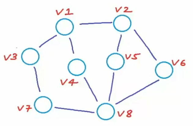
$|V|$: a number of vertices

$|E|$: a number of edges

Connection: Between two vertices, the connection can be directed or undirected.

Sometimes we gave edges weight. This graph is called weighted graph.

Walk: a sequence of vertices where each adjacent pair is connected by an edge.

Path: a walk in which no vertices (and thus no edges) are repeated.

Trail: a walk in which no edges are repeated.

Strong connected graphs: For a directed graph, if there is a path from any vertex to any other vertex.

Closed walk: a walk starts and ends at same vertex.

Simple cycle: no repetition other than start and end.

Acyclic graph: a graph with no cycle, like a tree.

How to store a graph

Vertex and edge list

We use string to store the vertex name. Use dynamic arrays to store the edges and the their weights.

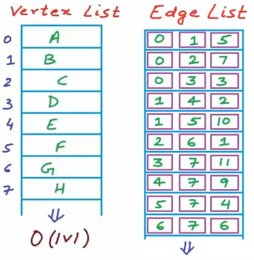
But this maybe cause costly time complexity.

Operation	Time Complexity
Finding adjacent nodes	$O(|E|)=O(v^2) \rightarrow costly$
Check if given nodes are connected	$O(|E|)=O(v^2) \rightarrow costly$

Adjacency Matrix

We use a vertex list and an adjacency matrix to store a graph.

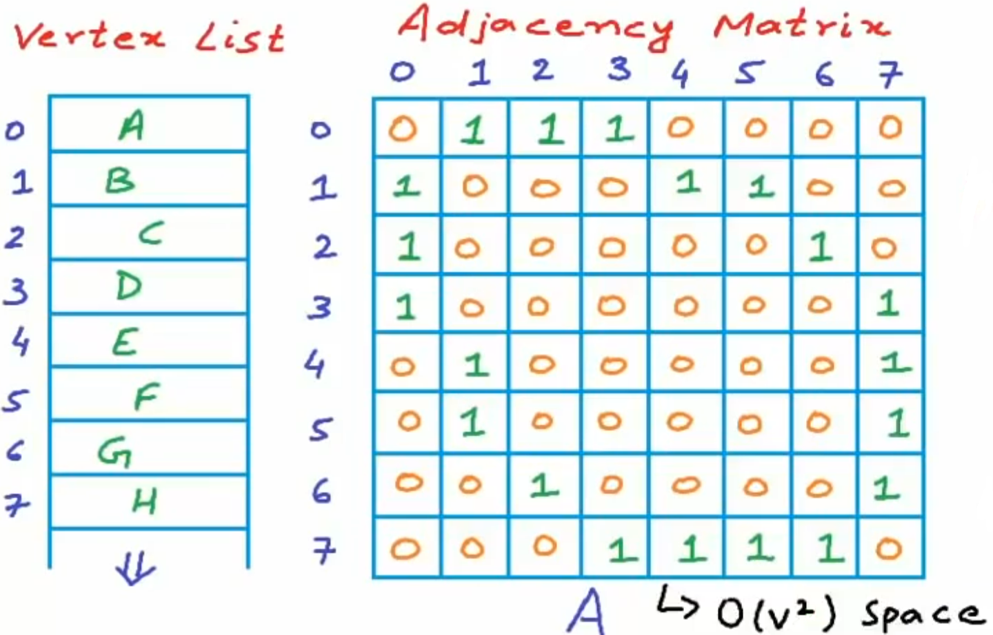
The elements in the adjacency matrix are defined as below.

$$A_{ij} = \left\{ \begin{matrix} 0, & \text{if}\,\exists\, \text{edge from i to j}\\ 1, & \text{otherwise} \end{matrix}\right.$$

For the weighted graph, the $A_{ij}$ will be defined as below.

$$A_{ij} = \left\{ \begin{matrix} \omega, & \text{if}\,\exists\, \text{edge from i to j}\\ \infty, & \text{otherwise} \end{matrix}\right.$$

Operation	Time Complexity
Finding adjacent nodes	$O(v)$
Check if given nodes are connected	$O(1)$(Use hash table to match the vertex name with its index)

We effectively reduce the time-cost, but take huge space-cost. In this method, the unconnected edge information is redundant. If the graph is dense, this method may be effective, but if the graph is sparse, a amount of the space is wasted. While most graph in the reality is sparse, that is the number of edges is much smaller than the square of the number of the vertices.

Adjacency list representation

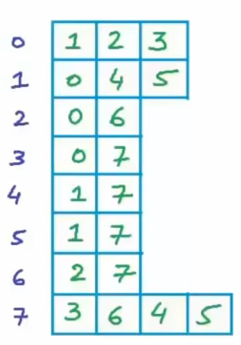
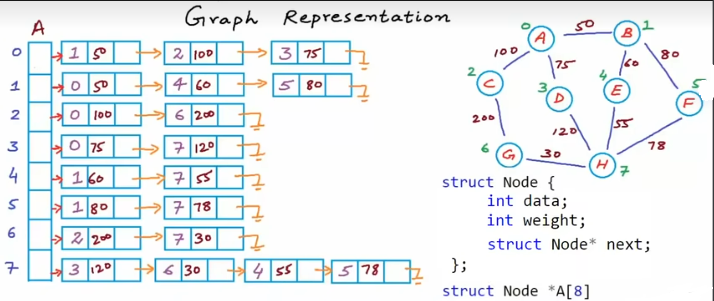
Instead of storing whether the node is connected or not, we choose to store the index of which nodes the targeted node connects to. Showed in the above figure, the first row represents the zeroth node connects to the first, the second and the third node. Specifically, what is the first node? We can search it in the Vertex List. So, by building adjacency list, we can reduce the space complexity from $O(v^2)$ to $O(e)$, which is the smallest memory consumption because in the realistic world, the most graphs are sparse, $|E|<<|V|^2$. We can use pointer to store the adjacency in C++ like the code below.

int *A[8];
A[0] = new int[3];
A[1] = new int[3];
A[2] = new int[2];
...
A[7] = new int[4];

You can use A array to store eight pointers. Each pointer points to a integral array, which stores indices the targeted node connects to.

Operation	Time Complexity
Finding adjacent nodes	$O(v)$
Check if given nodes are connected	$O(v)$—by linear search
$O(log_2v)$— by binary search

It looks like we don’t save the time by using adjacency list, but the time complexity is calculated in the worst performance. If the matrix is much sparse, the difference between two method will show.

Moreover, if we want to store, insert or delete some elements, the array maybe ineffective. Linked List can be used to store data dynamically. And if we wanna store a weighted graph, we just need to change the linked list structure, such as create a new cell to store a weight, matched with the node. Furthermore, if we want to enhance the performance of the adjacency list, we can use the binary search tree to replace the linked list. That will be more interesting!!

Application

Dijkstra Algorithm

We don't offer what the Dijkstra Algorithm is here. It's rebundant. Let's talk about some details in the implementation. Here is the implementation of Dijkstra in Python.

def find_lowest_cost_node(node_costs: dict):
    lowest_cost = float("inf")
    lowest_cost_node = None
    for node in node_costs.keys():
        cost = node_costs[node]
        if cost < lowest_cost and node not in processed_nodes:
            lowest_cost = cost
            lowest_cost_node = node
    return lowest_cost_node


def dijkstra(graph: dict, node_costs: dict, node_parents: dict):
    lowest_costnode: str = find_lowest_cost_node(node_costs=node_costs)
    while lowest_costnode is not None:
        current_cost = node_costs[lowest_costnode]
        neighbor_node_costs: dict | int = graph[lowest_costnode]
        for neighbor_node in neighbor_node_costs.keys():
            new_cost = current_cost + neighbor_node_costs[neighbor_node]
            if node_costs[neighbor_node] > new_cost:
                node_costs[neighbor_node] = new_cost
                node_parents[neighbor_node] = lowest_costnode
        processed_nodes.append(lowest_costnode)
        lowest_costnode = find_lowest_cost_node(node_costs)
    return node_costs, node_parents

For input paraments, we need to offer the graph, the costs, and the parents. We use adjacency list or called hash table, which python implemented it with dictionary, to represent a graph. You will see a example below. And we need to a cost list called node_costs and a parent list called node_parents to update current cost and parent of each node.

Example:

# Define a cost hash table
node_costs = {}
node_costs["a"] = 6
node_costs["b"] = 2
node_costs["end"] = float("inf")

# Define a parents hash table
node_parents = {}
node_parents["a"] = "start"
node_parents["b"] = "start"
node_parents["end"] = None

In the subsequent process, we need to update the node_costs and node_parents, according to the caculation result. Here is a example:

# Define a graph
graph = {}
graph["start"] = {}
graph["start"]["a"] = 6
graph["start"]["b"] = 2
graph["a"] = {}
graph["a"]["end"] = 1
graph["b"] = {}
graph["b"]["a"] = 3
graph["b"]["end"] = 5
graph["end"] = {}

# Define a cost hash table
node_costs = {}
node_costs["a"] = 6
node_costs["b"] = 2
node_costs["end"] = float("inf")

# Define a parents hash table
node_parents = {}
node_parents["a"] = "start"
node_parents["b"] = "start"
node_parents["end"] = None

processedNodes = []

cost, parent = dijkstra(graph, nodeCosts, nodeParents)
print(cost, parent)

output：

{'a': 5, 'b': 2, 'end': 6} {'a': 'b', 'b': 'start', 'end': 'a'}

z1=2*sin(pi*85/180)/(1+exp(1)^2)
x=[2 1+2i;0.45 5]
z2=1/2.*log(x+sqrt(1+x.^2))
a=[-3:0.1:3]
z3=(exp(0.3.*a)-exp(-0.3.*a))/2.*sin(pi.*(0.3+a)/180)+log((0.3+a)./2)